Expressive GNNs and How To Tame Them
Published:
This blog post consists of research I’m currently engaged with at NUS. My findings span the past half-year’s worth of reading the literature and I’m excited to explain these concepts to you from scratch!
Foreword
At NUS, I’m currently looking into Graph Neural Network expressiveness and I’m really excited about it. I’ve spoken to a few seniors in this area and have learned so much over the past few months. It’s an exciting line of research within Graph DL and I’m sure the pace will pick up soon. It’s more theoretical than practical currently but there’s definitely room for expansion. In fact, I’m currently looking into the practical aspects of expressiveness at NUS, which seems to be an underexplored niche.
Before we get into the meat of the topic, let’s get some preliminaries off the list first!
Graph Neural Networks
Graphs
A graph is a data structure consists of nodes/vertices \(V\) and edges \(E\). These nodes represent entities or objects and the edges between them denote some relationship. These relationships are either unidirectional or bidirection. Let’s assume we’re working with undirected graphs for the rest of this post.
Graph Neural Networks
A graph \(\mathcal{G}(V, E)\) consists of vertices (or nodes) \(v \in V\) and edges \(e_{ij} \in E \subseteq {V \times V}\) joining two nodes \(i\) and \(j\). \(e_{i,j} = 1\) if there’s a connection between nodes \(i\) and \(j\), 0 otherwise. The neighbourhood of a node \(i\), namely \(\mathcal{N}_i\), is a defined as the set of all nodes with outgoing edges to and incoming edges from \(i\); formally, \(\mathcal{N}_i = \{j : e_{ij} \in E\}\).
Each node \(i\) has an associated representation \(h_i^t \in \mathbb{R}^n\) and (discrete or continuous) label \(y\), for each GNN layer \(t \in \{1, \dots, T\}\). Each node \(i\) starts off with \(h_i^1 = x_i\), where \(x_i \in \mathbb{R}^n\) is the input features for the node. Edges \(e_{ij}\) can also have an associated representation \(a_{ij}^t \in \mathbb{R}^m\) depending on context. Each GNN layer \(t\) performs a single step of Message Passing. This involves combining the target node representation \(h^{t}_i\) with the node representations \(h_j^{t}\) from the neighbourhood \(\mathcal{N}_i\) (Equation \ref{mp}). Intuitively, at a layer \(t\), the GNN looks at the \(t\)-hop neighbourhood of \(i\), represented by a subtree rooted at node \(i\).
\[\begin{equation} \label{mp} h^{t+1}_i = \sigma(\psi(h^{t}_i,~\square(\{h^t_j : j \in \mathcal{N}_i\}))) \end{equation}\]Here, \(\psi\) is any affine transformation function (like a MLP) and \(\sigma\) is a non-linear, element-wise activation function (like Sigmoid, ReLU, or Softmax. \(\square\) is a permutation-invariant aggregation function that combines neighbouring node features; choices include “sum”, “max”, “min”, and “mean”. This aggregation function can be thought of as a hashing function that operates on multisets (sets with legal repetition) of node features. The same can be done to edge representation \(a_{ij}^t\) (Equation \ref{edge_mp}):
\[\begin{equation} \label{edge_mp} a_{ij}^{t+1} = \phi(a_{ij}^t, h^t_i, h^t_j) \end{equation}\]\(\phi : \mathbb{R}^m \rightarrow \mathbb{R}^m\), parameterised by \(\theta\), takes in current edge feature \(a_{ij}^t\), and respective node features \(h^t_i\) and \(h^t_j\), to output the new edge representation \(a_{ij}^{t+1}\) for the next layer.

Figure 1: A node \(i\) has a feature vector \(x_i \in \mathbb{R}^n\) (coloured envelope) and has a neighbourhood \(\mathcal{N}_i\) (left). A single round of Message Passing involves aggregating (collecting) representations from a target node’s neighbourhood and incorporating them into its own representation, for all nodes in the graph in parallel (right).

Figure 2: (a) is the original graph. (b) is the rooted subtree of target node (green) at layer \(t=1\). (c) is the rooted subtree of target node (green) at layer \(t=2\). These rooted subtrees are multisets of node features.
Understanding Expressiveness
Expressiveness refers to the ability of a GNN to discriminate two graphs. The inability to learn structural information from graphs results in over-smoothing – when two different nodes are assigned the same embedding representation in latent space, thereby being classified as the same. Therefore, structural awareness is important as it imbues inductive biases such as invariance to positions of nodes into the GNN, thereby allowing it to tell apart graphs. This brings us to the concept of graph isomorphism.
Graph Isomorphism
Formally, two graphs are isomorphic if there exists a bijection (1:1 mapping) between its edges. This means the connectivities of the graphs should be alike. Trivially, if they are different, the two graphs are non-isomorphic.
Weisfeiler-Leman GI Test
Two graphs are isomorphic if there exists a bijection between the vertex sets of both graphs. As such, the most notable algorithm for graph isomorphism is the Weisfeiler-Leman (WL) test. All nodes are assigned an initial colour (node-wise discrete label) and through iterations of naive vertex refinement, the colours of nodes are updated by incorporating it with the colours of neighbouring nodes. This is done using a hash function that takes in a multiset of neighbouring node colours that outputs a unique label for the next round of refinement. The test determines two graphs are non-isomorphic if the distribution of new colours differ at some iteration. To ensure the WL test can really tell apart graphs, we need to ensure the hash function is injective (unique mapping from multiset to hashed value).

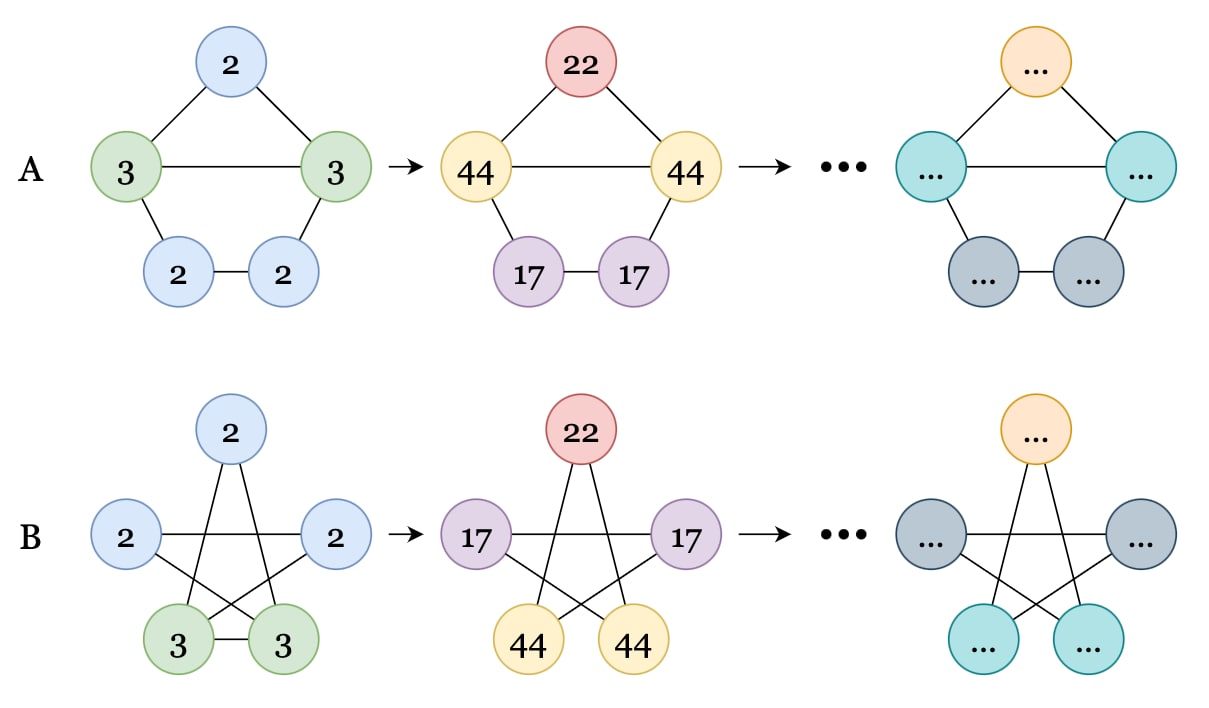
Figure 3: The WL test performed on two graphs \(A\) and \(B\) that are isomorphic. Labels are the degrees of each node. The multiset hashing function is \(H(S) = \sum_{i \in S} i^2\). Similar degree nodes are coloured the same to show that they get mapped to the same hash value. Notice how the distributions of node labels stay the same for the two graphs for all \(n\) iterations. This indicates they are highly likely isomorphic.
However, the WL test is necessary but insufficient to show graph isomorphism as there exist pairs of non-isomorphic graphs that are indistinguishable using the method. However, it has been a reliable test so far and works on most graphs.

Figure 4: Examples of two graphs indistinguishable by the WL test. They produce similar distributions through the iterations of colour refinement. It’s catastrophic if datasets have graphs that exhibit similar properties and can’t be told apart.
WL Test and Graph Neural Networks
In fact, we can draw parallels between the WL Test and a GNN. The aggregation function stays the same (simply collect neighbours’ labels) while the multiset hash function becomes the node readout function. Now, instead of node colours, we work with node features in GNNs. GNNs capable of discriminating two nodes (i.e., give them different representations in the embedding space) are at most as powerful as the WL Test (upper bound on expressiveness). Moreover, if we make the hash function/aggregation injective, the GNN can be as powerful as the WL Test (lower bound on expressiveness). This ensures two nodes are not assigned the same representation in the embedding space, thereby minimising the risk of classifying them as the same.
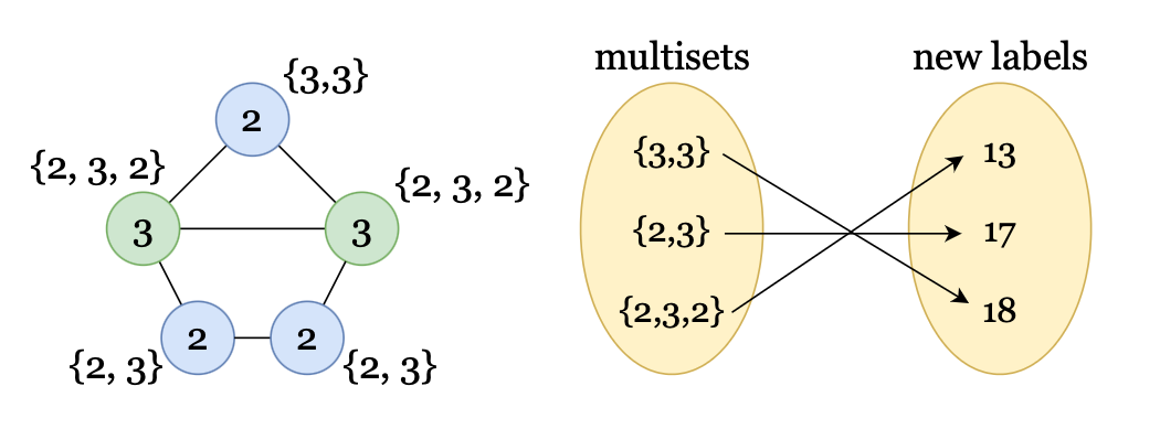
Figure 5: Mathematically, an injective function ensures that every possible output (in the codomain) has at most one associated input (in the domain) that results in said output. So, by introducing injectivity into aggregation/readout function, we ensure every node’s post-aggregation multiset is mapped to a unique label for the next iteration. Note that we aren’t taking the nodes’ own labels in the respective multisets.
Higher-Order Structures
So far, we’ve seen the WL test being used to discriminate between single nodes based on their colours/labels. There are more complex structures within graphs that can be used to tell apart said graphs. Examples of these higher-order structures include rooted subtrees, \(k\)-hop neighbourhoods, and pairs/tuples of connected nodes. The more expressive a GNN, the better it can make use of these structural hints (i.e., these higher-order structures) to discriminate graphs during training.
In fact, certain works in the literature even augment GNNs with this higher-order structural information that cannot directly be inferred through the simple WL test.
Weisfeiler-Leman Hierarchy
The vanilla WL test examines individual nodes and looks at their immediate 1-hop neighbourhood. GNNs capable of discerning graphs using this 1-hop neighbourhood are called 1-WL GNNs. More formally, we say the GNN is as powerful as 1-WL. We can generalise this to the \(k\)-hop neighbourhood where \(k \in \{2, 3, \dots\}\). This wider neighbourhood can be viewed as a larger multiset of neighbours and their neighbours, forming so-called higher-order structures. When a GNN is able to discern these higher-order structures, we call it a \(k\)-WL GNN, and claim the GNN is as powerful as \(k\)-WL. Expressiveness is measured using these different “levels” of \(k\)-WL, altogether forming the WL Hierarchy. A \(k\)-WL GNN is strictly weaker than a $(k+1)$-WL GNN in that there exists a graph that the latter can discriminate while the former cannot but the converse is not true.

Figure 6.1: Expressiveness is quantitatively defined using the WL Hierarchy. (top left) is the original graph. (top right) shows 1-WL expressiveness using the immediate 1-hop neighbourhood. The gray rectangles are the aggregated messages from the immediate neighbours. This is rather trivial.
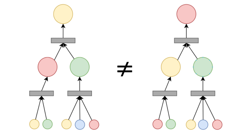
Figure 6.2: Here, I show 2-WL expressiveness using the 2-hop neighbourhood.
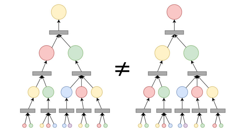
Figure 6.3: Likewise, here, I show 3-WL expressiveness using the 3-hop neighbourhood.
The objective is discriminate both graphs (hence the \(\neq\)) despite their structures being the same. Altogether, they form rooted subtrees w.r.t. the target nodes being compared.
In fact, regular Message Passing Neural Networks fail 1-WL because aggregation functions like “mean” and “max” cannot tell apart two non-identical graphs. To avoid such scenarios, we introduce injectivity to the aggregation (multiset hashing) function; the “sum” aggregator is one such example.
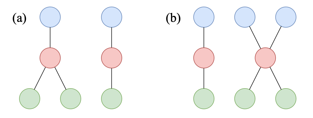
Figure 7: The graphs on the left cannot be discriminated using the “max” aggregator. The graphs on the right cannot be discriminated using the “max” and “mean” aggregators. This is because these functions are not injective by nature.
Conclusion
The theoretical research community has more or less moved away from standard GNNs towards expressive GNNs like those mentioned above. The obvious benefits include better structural awareness, which is paramount for real-life problems like protein studies, molecule interaction modelling, and social media analysis. I hope this blogpost shares some exciting insights about this new family of expressive GNNs. In terms of what’s to come, I believe we need more benchmarking efforts to really compare these expressive GNNs with one another. This means coming up with new, dedicated datasets, both real-life and synthetic.
Let me know if you want an in-depth review of notable works from the literature; there have been a lot of exciting SOTA works coming out lately. Also let me know if you want to access the extensive reading list I used to get me up-to-speed.
I look forward to sharing more with you in time! Lots of exciting work to be done and lots of learnings and takeaways in store. Stay tuned!
Till then, I’ll see you in the next post :D
