
Math Behind Graph Neural Networks
Published:
Foreword
I’ve heard numerous requests to write something like this. The following blog post is my humble attempt at bridging the gaps in Graph Deep Learning. Don’t worry, I’ve added tons of diagrams and drawings to help visualise the whole thing! Also, I explicitly avoid the actual math-heavy concepts like spectral graph theory. Maybe an article for the future! The bulk of this article is comprehensive as long as you know the very basics of regular Machine Learning.
Preface
Graph Deep Learning (GDL) has picked up its pace over the years. The natural network-like structure of many real-life problems makes GDL a versatile tool in the shed. The field has shown a lot of promise in social media, drug-discovery, chip placement, forecasting, bioinformatics, and more.
Here, I wish to provide a breakdown of popular Graph Neural Networks and their mathematical nuances – a very tiny survey, of sorts. Think of this as the continuation to my previous article on Graph Neural Networks that had no math at all.
⭐ The idea behind Graph Deep Learning is to learn the structural and spatial features over a graph with nodes and edges that represent entities and their interactions.
Structure of this article
I start off by providing an in-depth breakdown of Graphs and Graph Neural Networks. Here, I deep dive into the granular steps one would take for the forward pass. Then, I move on to training these networks using familiar end-to-end techniques. Finally, I use the steps in the forward pass section as a framework or guideline to introduce popular Graph Neural Networks from the literature.
- Foreword
- Preface
- Representing Graphs
- Graph Neural Networks
- Message Passing
- Stacking GNN layers
- Training a GNN (context: Node Classification)
- Popular Graph Neural Networks
- Conclusion
Representing Graphs
Before we get into Graph Neural Networks, let’s explore what a graph is in Computer Science.
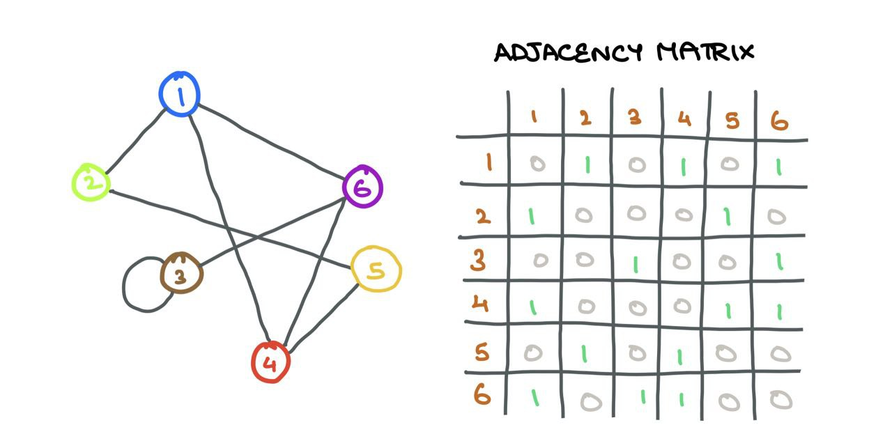
A graph \(\mathcal{G}(V, E)\) is a data structure containing a set of vertices (nodes) \(i \in V\)and a set of edges \(e_{ij} \in E\) connecting vertices \(i\) and \(j\). If two nodes \(i\) and \(j\) are connected, \(e_{ij} = 1\), and \(e_{ij} = 0\) otherwise. One can store this connection information in an Adjacency Matrix \(A\):
⚠️ I assume the graphs in this article are unweighted (no edge weights or distances) and undirected (no direction of association between nodes). I assume these graphs are homogenous (single type of nodes and edges; opposite being “heterogenous”).
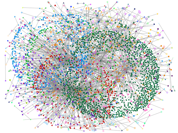
Graphs differ from regular data in that they have a structure that neural networks must respect; it’d be a waste not to make use of it. Here’s an example of a social media graph where nodes are users and edges are their interactions (like follow/like/retweet).
Connection to Images
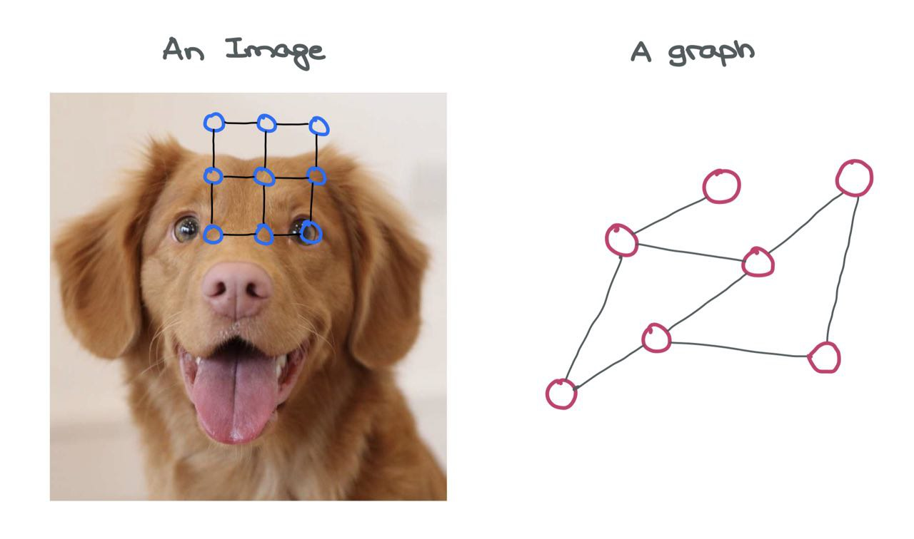
An image is a graph on its own! It’s a special variant called a “Grid Graph” where the number of outgoing edges from a node is constant for all internal and corner nodes. There’s some consistent structure present in the image grid graph that allows for simple Convolution-like operations to be performed on it.
An image can be considered a special graph where each pixel is a node and is connected to other pixels around it via imaginary edges. Of course, it’s impractical to view images in this light as that would mean having a very large graph. For instance, a simple CIFAR-10 image of \(32 \times 32 \times 3\) would have \(3072\) nodes and 1984 edges. For larger ImageNet images of \(224 \times 224 \times 3\), these numbers would blow up.
An image can be considered a special graph where each pixel is a node and is connected to other pixels around it via imaginary edges. Of course, it’s impractical to view images in this light as that would mean having a very large graph. For instance, a simple CIFAR-10 image of \(32 \times 32 \times 3\) would have \(3072\) nodes and 1984 edges. For larger ImageNet images of \(224 \times 224 \times 3\), these numbers would blow up.
However, as you can observe, a graph isn’t that perfect. Different nodes have different degrees (number of connections to other nodes) and is all over the place. There is no fixed structure but the structure is what adds value to the graph. So, any neural network that learns on this graph must respect this structure while learning the spatial relationships between the nodes (and edges).
😌 As much as we want to use image processing techniques here, it’d be nice to have special graph-specific methods that are efficient and comprehensive for both small and large graphs.
Graph Neural Networks
A single Graph Neural Network (GNN) layer has a bunch of steps that’s performed on every node in the graph:
- Message Passing
- Aggregation
- Update
Together, these form the building blocks that learn over graphs. Innovations in GDL mainly involve changes to these 3 steps.
What’s in a Node?
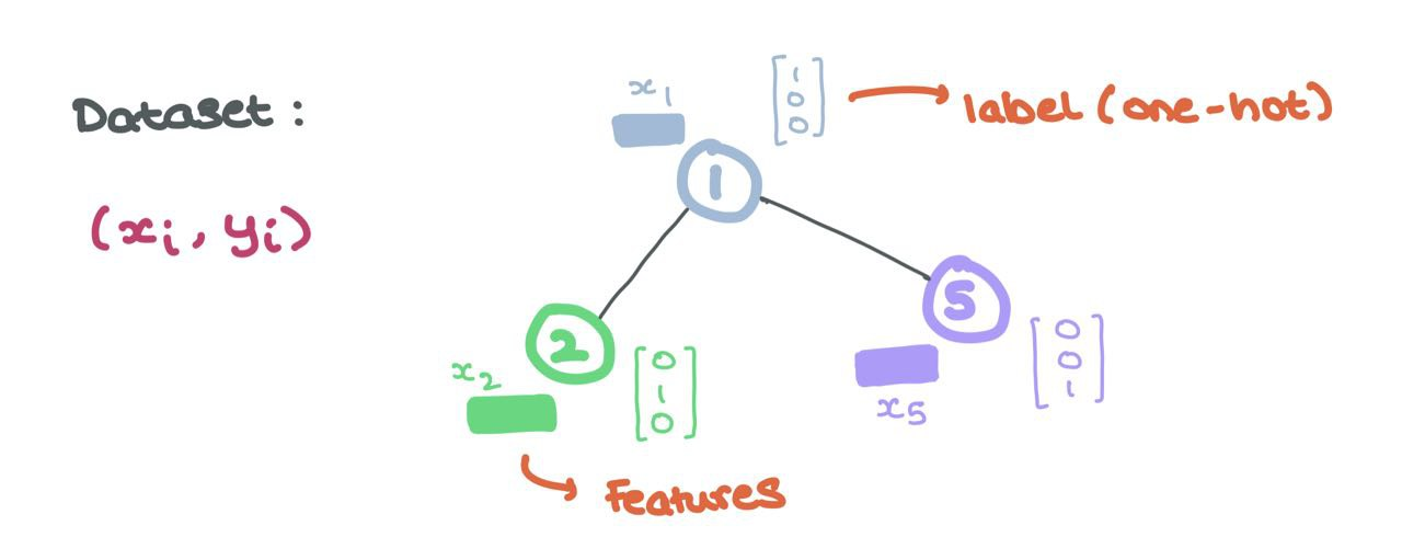
Remember: a node represents an entity or object, like a user or atom. As such, this node has a bunch of properties characteristic to the entity being represented. These node properties form the features of a node (i.e., “node features” or “node embeddings”).
Typically, these features can be represented using vectors in \(\mathbb{R}^d\). This vector is either a latent-dimensional embedding or is constructed in a way where each entry is a different property of the entity.
🤔 For instance, in a social media graph, a user node has the properties of age, gender, political inclination, relationship status, etc. that can be represented numerically.
Likewise, in a molecule graph, an atom node might have chemical properties like affinity to water, forces, energies, etc. that can also be represented numerically.
These node features are the inputs to the GNN as we will see in the coming sections. Formally, every node \(i\) has associated node features \(x_i \in \mathbb{R}^d\) and labels \(y_i\) (that can either be continuous or discrete like one-hot encodings).
Edges Matter Too!!!
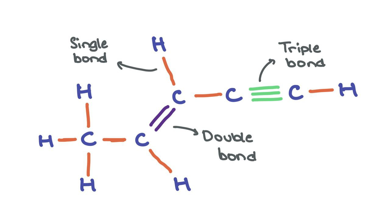
Edges can have features \(a_{ij} \in \mathbb{R}^{d^\prime}\) as well, for instance, in cases where edges have meaning (like chemical bonds between atoms). We can think of the molecule shown below as a graph where atoms are nodes and bonds are edges.
While the atom nodes themselves have respective feature vectors, the edges can have different edge features that encode the different types of bonds (single, double, triple). Though, for the sake of simplicity, I’ll be omitting edge features in the following article.
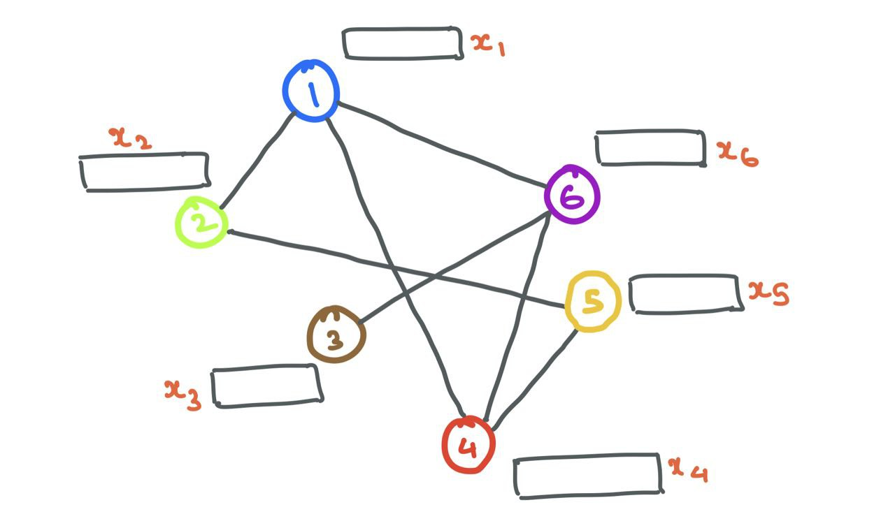
Now that we know how to represent nodes and edges in a graph, let’s start off with a simple graph with a bunch of nodes (with node features) and edges.
Message Passing
GNNs are known for their ability to learn structural information. Usually, nodes with similar features or properties are connected to each other (this is true in the social media setting). The GNN exploits this fact and learns how and why specific nodes connect to one other while some do not. To do so, the GNN looks at the Neighbourhoods of nodes.
The Neighbourhood \(\mathcal{N}_i\) of a node \(i\) is defined as the set of nodes \(j\) connected to \(i\) by an edge. Formally, \(\mathcal{N}_i = \{j ~:~ e_{ij} \in E\}\).
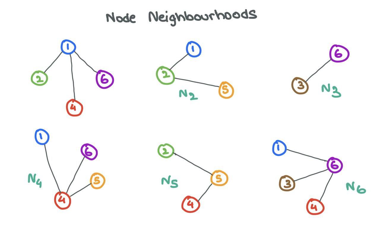
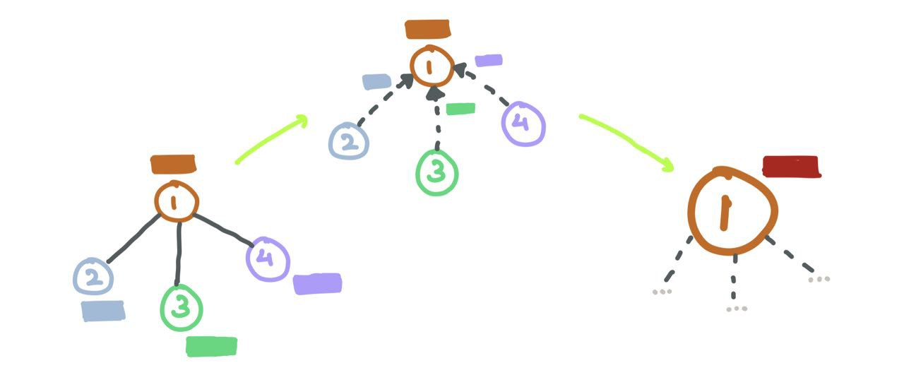
A person is shaped by the circle he is in. Similarly, a GNN can learn a lot about a node \(i\) by looking at the nodes in its neighbourhood \(\mathcal{N}_i\). To enable this sharing of information between a source node \(i\) and its neighbours \(j\), GNNs engage in Message Passing.
For a GNN layer, Message Passing is defined as the process of taking node features of the neighbours, transforming them, and “passing” them to the source node. This process is repeated, in parallel, for all nodes in the graph. In that way, all neighbourhoods are examined by the end of this step.
Let’s zoom into node \(6\) and examine the neighbourhood \(\mathcal{N}_6 = \{1,~3,~4\}\). We take each of the node features \(x_1\), \(x_3\), and \(x_4\), and transform them using a function \(F\), which can be a simple neural network (MLP or RNN) or affine transform \(F(x_j) = \mathbf{W}_j \cdot x_j + b\). Simply put, a “message” is the transformed node feature coming in from source node.
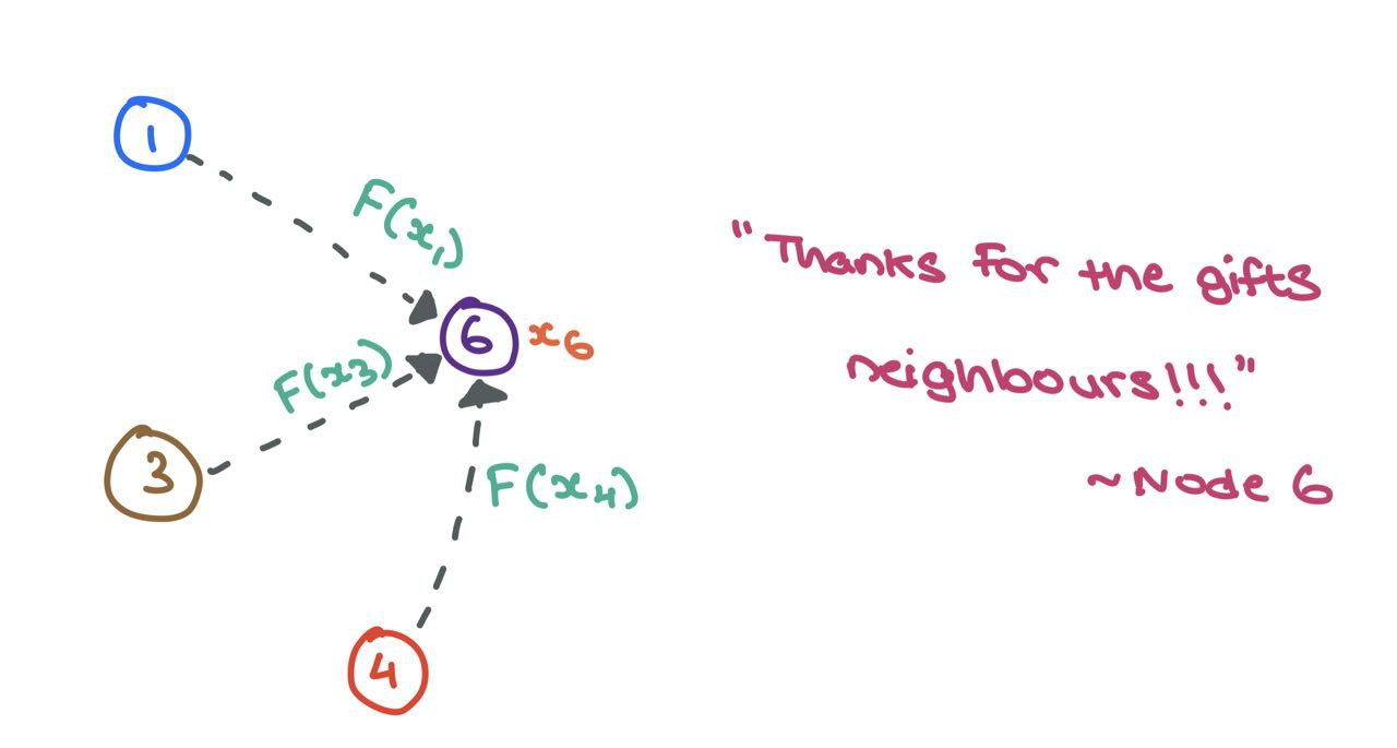 \(F\) can be a simple affine transform or neural network.
For now, let’s say \(F(x_j) = \mathbf{W}_j\cdot x_j\) for mathematical convenience. Here, \(\square \cdot \square\) represents simple matrix multiplication.
Aggregation
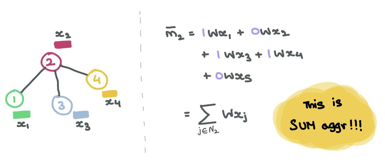
Now that we have the transformed messages \(\{F(x_1), F(x_3), F(x_4)\}\) passed to node \(6\), we have to aggregate (“combine”) them someway. There are many things that can be done to combine them. Popular aggregation functions include,
\[\begin{align} \text{Sum } &=\sum_{j \in \mathcal{N}_i} \mathbf{W}_j\cdot x_j \\ \text{Mean }&= \frac{\sum_{j \in \mathcal{N}_i} \mathbf{W}_j\cdot x_j}{|\mathcal{N}_i|} \\ \text{Max }&= \max_{j \in \mathcal{N}_i}(\{\mathbf{W}_j\cdot x_j\}) \\ \text{Min }&= \min_{j \in \mathcal{N}_i}(\{\mathbf{W}_j\cdot x_j\})\end{align}\]Suppose we use a function \(G\) to aggregate the neighbours’ messages (either using sum, mean, max, or min). The final aggregated messages can be denoted as follows:
\[\bar{m}_i = G(\{\mathbf{W}_j \cdot x_j : j \in \mathcal{N}_i\})\]Update
Using these aggregated messages, the GNN layer now has to update the source node \(i\)’s features. At the end of this update step, the node should not only know about itself but its neighbours as well. This is ensured by taking the node \(i\)’s feature vector and combining it with the aggregated messages. Again, a simple addition or concatenation operation takes care of this.
Using addition:
\[h_i = \sigma(K(H(x_i) + \bar{m}_i)))\]where \(\sigma\) is an activation function (ReLU, ELU, Tanh), \(H\) is a simple neural network (MLP) or affine transform, and \(K\) is another MLP to project the added vectors into another dimension.
Using concatenation:
\[h_i = \sigma(K(H(x_i) ~\oplus~ \bar{m}_i)))\]To abstract this update step further, we can think of \(K\) as some projection function that transforms the messages and source node embedding together:
\[h_i = \sigma(K(H(x_i),~ \bar{m}_i)))\]👉🏻 Notation-wise, the initial node features are called \(x_i\).
After a forward pass through the first GNN layer, we call the node features \(h_i\) instead. Suppose we have more GNN layers, we can denote the node features as \(h_i^l\) where \(l\) is the current GNN layer index. Also, it’s evident that \(h_i^0 = x_i\) (i.e., the input to the GNN).
Putting Them Together
Now that we’ve gone through the Message Passing, Aggregation, and Update steps, let’s put them all together to formulate a single GNN layer on a single node \(i\):
\[h_i = \sigma(W_1\cdot h_i + \sum_{j \in \mathcal{N}_i}\mathbf{W}_2\cdot h_j )\]Here, we use the sum aggregation and a simple feed-forward layer as functions \(F\) and \(H\).
⚠️ Do ensure that the dimensions of \(\mathbf{W}_1\) and \(\mathbf{W}_2\) commute properly with the node embeddings. If \(h_i \in \mathbb{R}^{d}\), \(\mathbf{W}_1, \mathbf{W}_2 \subseteq \mathbb{R}^{d^\prime \times d}\) where \(d^\prime\) is the embedding dimension.
Working with Edge Features
When working with edge features, we’ll have to find a way to a GNN forward pass on them. Suppose edges have features \(a_{ij} \in \mathbb{R}^{d^\prime}\). To update them at a specific layer \(l\), we can factor in the embeddings of the nodes on either side of the edge. Formally,
\[a^{l}_{ij} = T(h^l_i,~ h^l_j,~ a^{l-1}_{ij})\]where \(T\) is a simple neural network (MLP or RNN) that takes in the embeddings from connected nodes \(i\) and \(j\) as well as the previous layer’s edge embedding \(a^{l-1}_{ij}\).
Working with Adjacency Matrices
So far, we looked at the entire GNN forward pass through the lense of a single node \(i\) in isolation and its neighbourhood \(\mathcal{N}_i\). However, it’s also important to know how to implement the GNN forward pass when given a whole adjacency matrix \(A\) and all \(N = \|V\|\) node features in \(X \subseteq \mathbb{R}^{N \times d}\).
In normal Machine Learning, in a MLP forward pass, we want to weight the items in the feature vector \(x_i\). This can be seen as the dot product of the node feature vector \(x_i \in \mathbb{R}^d\) and parameter matrix \(W \subseteq \mathbb{R}^{d^\prime \times d}\) where \(d^\prime\) is the embedding dimension:
\[z_i = \mathbf{W} \cdot x_i ~~\in \mathbb{R}^{d^\prime}\]If we want to do this for all samples in the dataset (Vectorisation), we just matrix-multiply the parameter matrix and the features to get the transformed node features (messages):
\[\mathbf{Z} = (\mathbf{W}\mathbf{X} )^T = \mathbf{X}\mathbf{W} ~~\subseteq \mathbb{R}^{N \times d^\prime}\]Now, in GNNs, for every node \(i\), a message aggregation operation involves taking neighbouring node feature vectors, transforming them, and adding them up (in the case of sum aggregation).
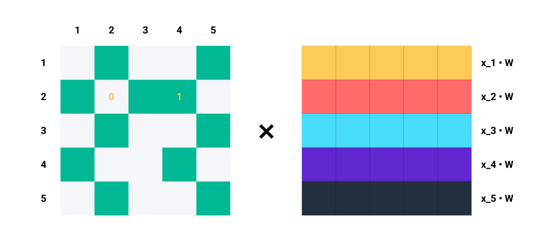
A single row \(A_i\) in the adjacency matrix tells us which nodes \(j\) are connected to \(i\). For every indiex \(j\) where \(A_{ij}=1\), we know node \(i\) and \(j\) are connected → \(e_{ij} \in E\).
For example, if \(A_2 = [1, 0, 1, 1, 0]\), we know that node \(2\) is connected to nodes \(1\), \(3\), and \(4\). So, when we multiply \(A_2\) with \(\mathbf{Z} = \mathbf{X}\mathbf{W}\) , we only consider the columns \(1\), \(3\), and \(4\) while ignoring columns \(2\) and \(5\). In terms of matrix multiplication, we are doing:
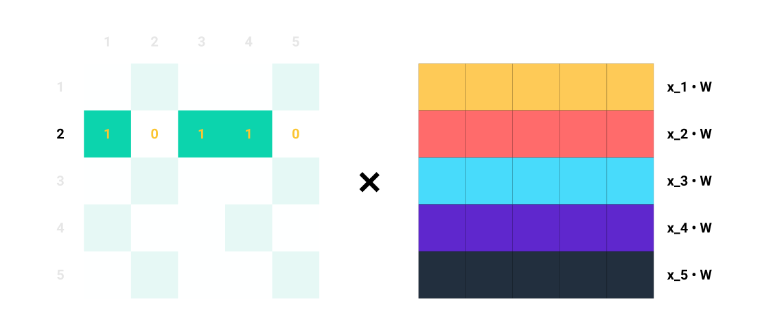 Let’s focus on row 2 of \(A\).
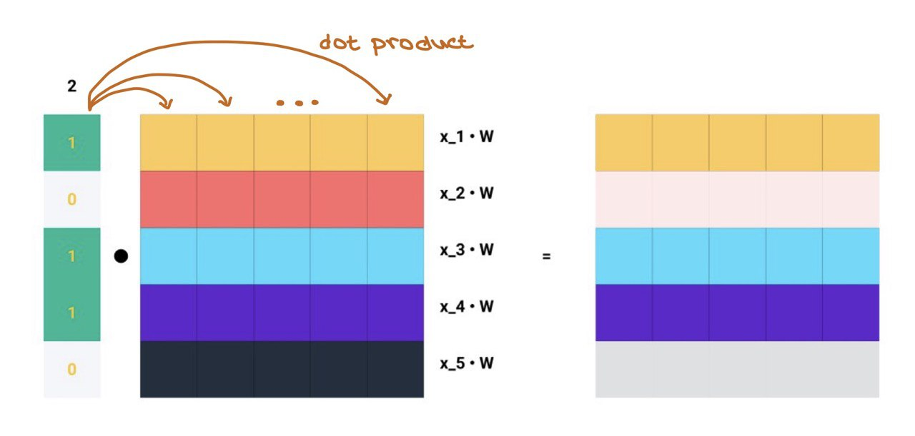
Matrix multiplication is simply the dot product of every row in \(A\) with every column in \(\mathbf{Z} = \mathbf{X}\mathbf{W}\)!!!
… and this is exactly what message aggregation is!!!
To get the aggregated messages for all \(N\) nodes in the graph based on their connections, we can matrix-multiply the entire adjacency matrix \(A\) with the transformed node features:
\[\text{Y} = AZ = AXW\]‼️ A tiny problem: Observe that the aggregated messages do not factor in node \(i\)’s own feature vector (as we did above). To do that, we add self-loops to \(A\) (each node \(i\) is connected to itself).
This means changing the \(0\) to a \(1\) at every position \(A_{ii}\) (i.e., the diagonals).
With some linear algebra, we can do this using the Identity Matrix!
\[\tilde{A} = A + I_{N}\]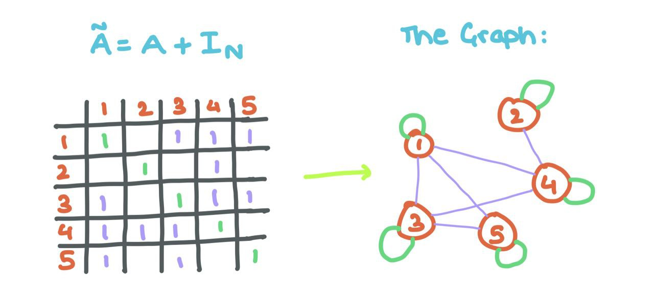
Adding self-loops allows the GNN to aggregate the source node’s features along with that of its neighbours!!
And with that, this is how you can do the GNN forward pass using matrices instead of single nodes.
⭐ To perform the mean aggregation, we can simple divide the sum by the count of \(1\)s in \(A_i\). For the example above, since there are three \(1\)s in \(A_2 = [1, 0, 0, 1, 1]\), we can divide \(\sum_{j \in \mathcal{N}_2}\mathbf{W}x_j\) by \(3\) … which is exactly the mean!!!
Though, It’s not possible to achieve max and min aggregation with the adjacency matrix formulation of GNNs.
Stacking GNN layers
Now that we’ve figured out how single GNN layers work, how we build a whole “network” of these layers? How does information flow between the layers and how the GNN refine the embeddings/representations of the nodes (and/or edges)?
- The input to the first GNN layer is the node features \(X \subseteq \mathbb{R}^{N \times d}\). The output is the intermediate node embeddings \(H^1 \subseteq \mathbb{R}^{N \times d_1}\) where \(d_1\) is the first embedding dimension. \(H^1\) is made up of \(h^1_{i ~:~ 1 \rightarrow N} \in \mathbb{R}^{d_1}\).
- \(H^1\) is the input to the second layer. The next output is \(H^2 \subseteq \mathbb{R}^{N \times d_2}\) where \(d_2\) is the second layer’s embedding dimension. Likewise, \(H^2\) is made up of \(h^2_{i ~:~ 1 \rightarrow N} \in \mathbb{R}^{d_2}\).
- After a few layers, at the output layer \(L\), the output is \(H^L \subseteq \mathbb{R}^{N \times d_L}\). Finally, \(H^L\) is made up of \(h^L_{i ~:~ 1 \rightarrow N} \in \mathbb{R}^{d_L}\).
The choice of \(\{d_1, d_2,\dots,d_L\}\) is completely up to us and are hyperparameters of the GNN. Think of these as choosing units (number of “neurons”) for a bunch of MLP layers.
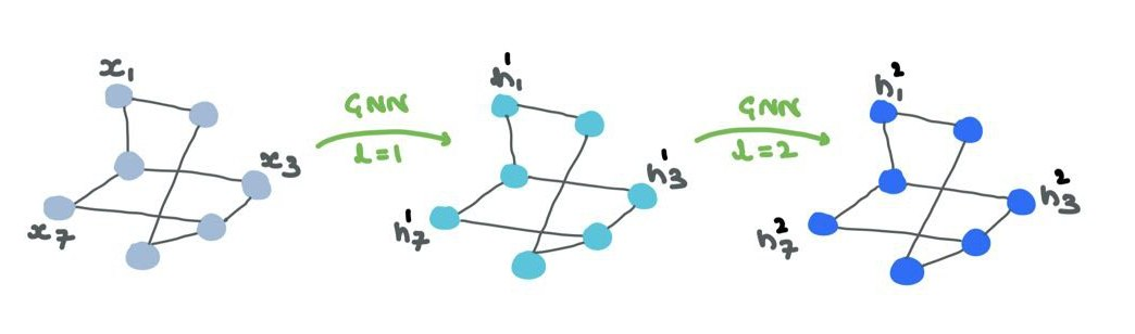
The node features/embeddings (“representations”) are passed through the GNN. The structure remains the same but the node representations are constantly changing through the layers. Optionally, your edge representations will also change but will no change connections or orientation.
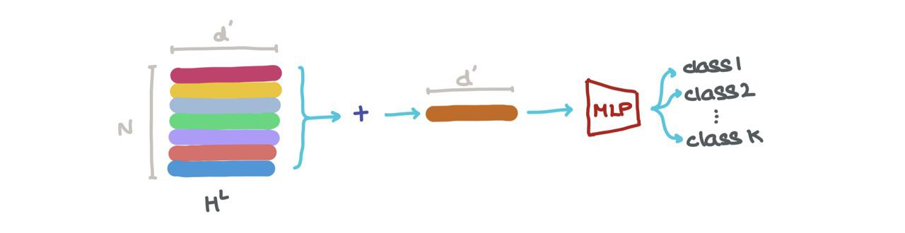
Now, there are a few things we can do with \(H^L\):
- We can add it along the first axis (i.e., \(\sum_{k=1}^N h_k^L\)) to get a vector in \(\mathbb{R}^{d_L}\). This vector is the latest dimensional representation of the whole graph. It can be used for graph classification (eg: what molecule is this?).
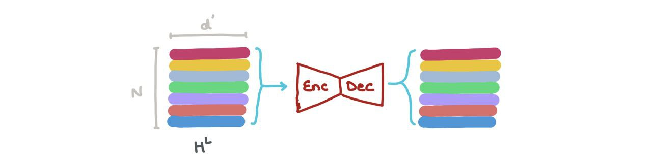
- We can concatenate the vectors in \(H^L\) (i.e., \(\bigoplus_{k=1}^N h_k\) where \(\oplus\) is the vector concatenation operation) and pass it through a Graph Autoencoder. This might help when the input graphs are noisy or corrupted and we want to reconstruct the denoised graph.
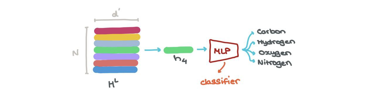
- We can do node classification → what class does this node belong to? The node embedding at a specific index \(h_i^L\) (\(i : 1 \rightarrow N\)) can be put through a classifier (like a MLP) into \(K\) classes (eg: is this a Carbon atom, Hydrogen atom, or Oxygen atom?).
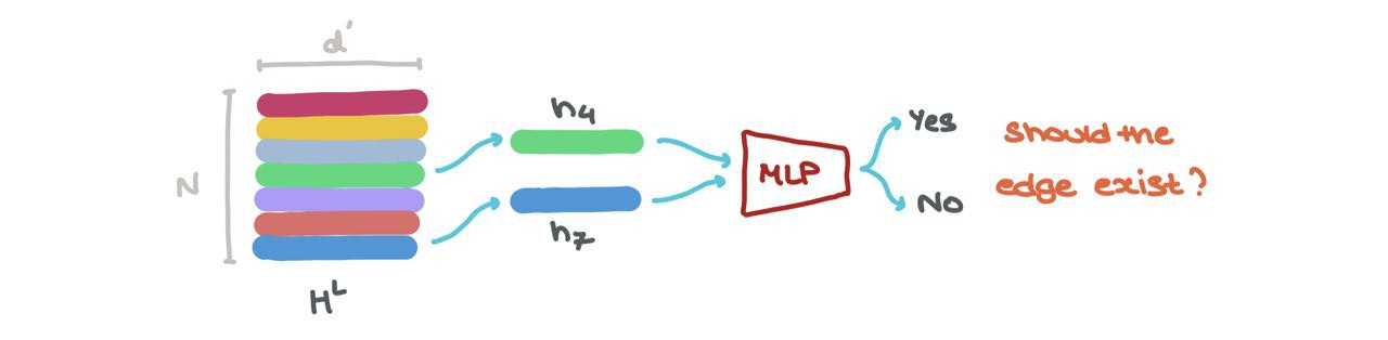
- We can perform link prediction → should there be a link between some node \(i\) and \(j\)? The node embeddings for \(h_i^L\) and \(h_j^L\) can be fed into another Sigmoid-based MLP that spits out a probability of an edge existing between those nodes.
Either way, the fun thing is, each \(h_{1 \rightarrow N} \in H^L\) can be stacked and thought of as a batch of samples. One can easily treat it as a batch.
🚨 For a given node \(i\), the \(l^{\text{th}}\) layer in the GNN aggregates features the \(l\)-hop neighbourhood of node \(i\). Initially, the node sees its immediate neighbours and deeper into the network, it interacts with neighbours’ neighbours and so on.
This is why, for very small, sparse (very few edges) graphs, a large number of GNN layers often leads to a degradation in performance. This is because the node embeddings all converge to a singular vector as each node has seen nodes many hops away. This is a useless situation to be in!!!
Which explains why most GNN papers often use \(\leq4\) layers for their experiments to prevent the network from dying.
Training a GNN (context: Node Classification)
🥳 During training, the predictions for nodes, edges, or the whole graph can be compared with the ground-truth labels from the dataset using a loss function (eg: Cross Entropy).
This enables GNNs to be trained in an end-to-end manner using vanilla Backprop and Gradient Descent.
Training and Testing Graph Data
As with regular ML, graph data can be split into training and testing as well. This can be done in one of two ways:
Transductive
The training and testing data are both present in the same graph. The nodes from each set are connected to one another. It’s just that, during training, the labels for the testing nodes are hidden while the labels for training nodes are visible. However, the features of ALL nodes are visible to the GNN.
We can do this with a binary mask over all the nodes (if a training node \(i\) is connected to a testing node \(j\), just set \(A_{ij} = 0\) in the adjacency matrix).
![]() In the transductive setting, training and testing nodes are both part of the SAME graph. Just that training nodes expose their features and labels while testing nodes only expose their features. The testing labels are hidden from the model. Binary masks are needed to tell the GNN what’s a training node and what’s a testing node.
In the transductive setting, training and testing nodes are both part of the SAME graph. Just that training nodes expose their features and labels while testing nodes only expose their features. The testing labels are hidden from the model. Binary masks are needed to tell the GNN what’s a training node and what’s a testing node.
Inductive
Here, there are separate training and testing graphs that are hidden from one another. This is akin to regular ML where the model only sees the features and labels during training, and only the features for testing. Training and testing take place on two separate, isolated graphs. Sometimes, these testing graphs are out-of-distribution to check for quality of generalisation during training.
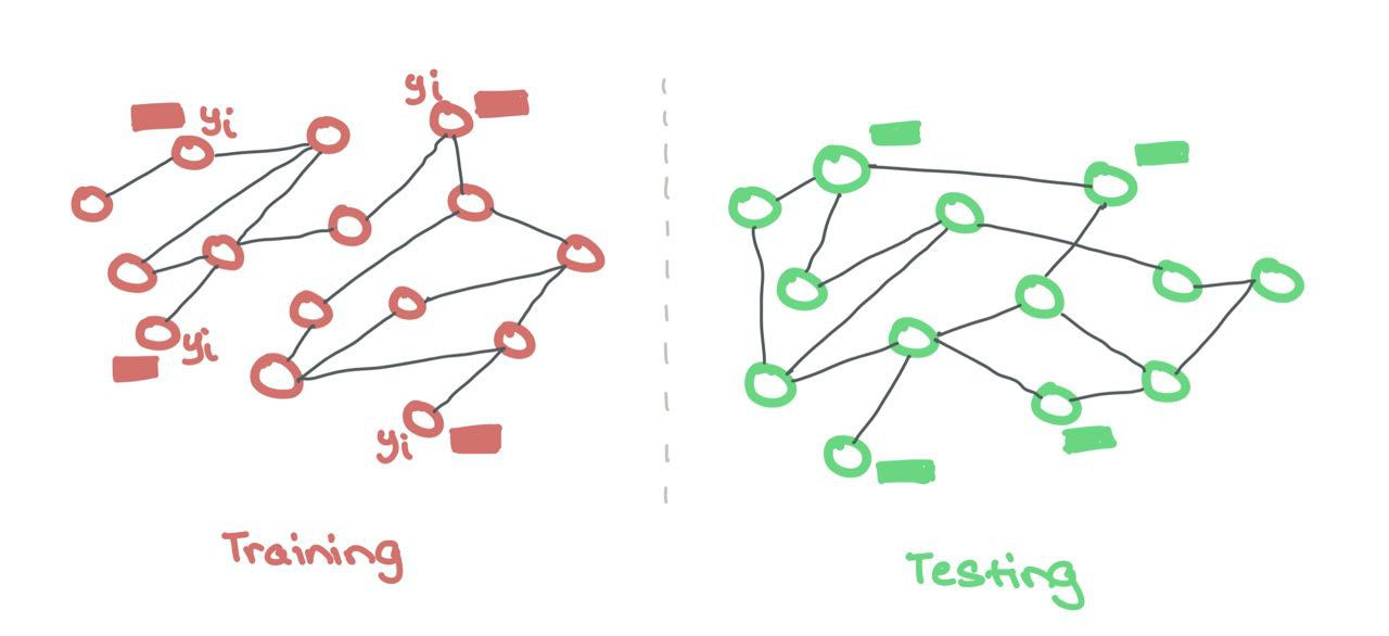
Like regular ML, the training and testing data are kept separately. The GNN makes use of features and labels ONLY from the training nodes. There is no binary mask needed here to hide the testing nodes as they are from a different set.
Backprop and Gradient Descent
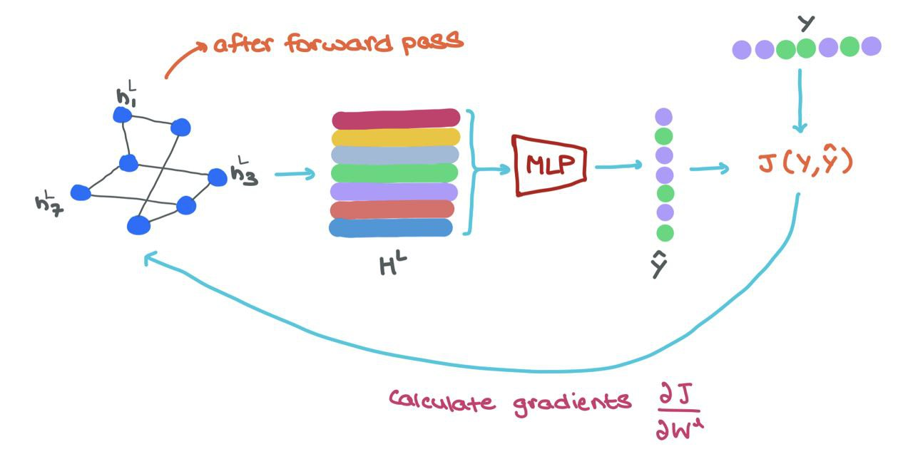
During training, once we do the forward pass through the GNN, we get the final node representations \(h^L_i \in H^L\). To train the network in an end-to-end manner, we can do the following:
- Feed each \(h^L_i\) into a MLP classifier to get prediction \(\hat{y}_i\)
- Calculate loss using ground-truth \(y_i\) and prediction \(\hat{y}_i\) → \(J(\hat{y}_i, y_i)\)
- Use Backpropagatino to compute gradients \(\frac{\partial J}{\partial W^l}\) where \(W^l\) is the parameter matrix from layer \(l\)
- Use some optimiser (like Gradient Descent) to update the parameters \(W^l\) for each layer in the GNN
- (Optional) You can finetune the classifier (MLP) network’s weights as well.
🥳 This means GNNs are easily parallelisable both in terms of Message Passing and Training. The entire process can be vectorised (as shown above) and performed on GPUs!!!
Popular Graph Neural Networks
In this section, I cover some popular works in the literature and categories their equations and math into the 3 GNN steps mentioned above (or at least I try). A lot of popular architectures merge the Message Passing and Aggregation steps into one function performed together, rather than one after the other explicitly. I try to decompose them in this section but for mathematical convenience, it’s best to see them as a singular operation!
I’ve adapted the notation of the networks covered in this section to make it consistent with that of this article.
Message Passing Neural Network
Neural Message Passing for Quantum Chemistry
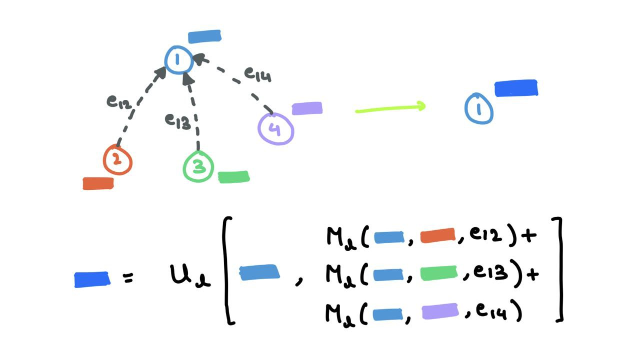
Message Passing Neural Networks (MPNN) decompose the forward pass into the Message Passing Phase with message function \(M_l\), and Readout Phase with vertex update function \(U_l\).
MPNN merges the Message Passing and Aggregation steps into the singular Message Passing Phase:
\[m_i^{l+1} = \sum_{j \in \mathcal{N}_i} M_l(h_i^l,~ h_j^l,~ e_{ij})\]The Readout Phase is the update step:
\[h_i^{l+1} = U_l(h_i^l,~ m_i^{l+1})\]where \(m_v^{l+1}\) is the aggregated message and \(h_v^{l+1}\) is the updated node embedding. This is very similar to the procedure I’ve mentioned above. The message function \(M_l\) is the mix of \(F\) and \(G\), and the function \(U_l\) is \(K\). Here, \(e_{ij}\) refers to possible edge features that can be omitted as well.
This paper uses MPNN as a general framework and formulate other works from the literature as special variations of a MPNN. The authors further use MPNN for quantum chemistry applications.
Graph Convolutional Network
Semi-Supervised Classification with Graph Convolutional Networks
The Graph Convolutional Network (GCN) paper looks at the whole graph in its adjacency matrix form. First, self-connections are added to the adjacency matrix to ensure all nodes are connected to themselves to get \(\tilde{A}\). This ensures we factor in the source node’s embeddings during Message Aggregation. The combined Message Aggregation and Update steps look like so:
\[H^{l+1} = \sigma(\tilde{A}H^lW^l)\]where \(W^l\) is a learnable parameter matrix. Of course, I change \(X\) to \(H\) to generalise the node features at ay arbitrary layer \(l\) where \(H^0 = X\).
🤔 Due to the associative property of matrix multiplication (\(A(BC) = (AB)C\)), it doesn’t matter which sequence we mutiply the matrices in (either \(\tilde{A}H^l\) first, post-multiply \(W^l\) next OR \(H^lW^l\) first, pre-multiply \(\tilde{A}\) next).
However, the authors, Kipf and Welling, further introduce a degree matrix \(\tilde{D}\) as a form of renormalisation to avoid numerical instabilities and exploding/vanishing gradients:
\[\tilde{D}_{ii} = \sum_j \tilde{A}_{ij}\]The “renormalisation” is carried out on the augmented adjacency matrix \(\hat{A} = \tilde{D}^{-\frac{1}{2}}\tilde{A}\tilde{D}^{-\frac{1}{2}}\). Altogether, the new combined Message Passing and Update steps look like so:
\[H^{l+1} = \sigma(\hat{A}H^lW^l)\]Graph Attention Network
Aggregation typically involves treating all neighbours equally in the sum, mean, max, and min settings. However, in most situations, some neighbours are more important than others. Graph Attention Networks (GAT) ensure this by weighting the edges between a source node and its neighbours using of Self-Attention by Vaswani et al. (2017).
Edge weights \(\alpha_{ij}\) are generated as follows.
\[\alpha_{ij} = \text{Softmax}(\text{LeakyReLU}(\mathbf{W_a}^T \cdot [\mathbf{W}h^l_i ~\oplus~ \mathbf{W}h^l_j]))\]where \(\mathbf{W_a} \in \mathbb{R}^{2d^\prime}\) and \(\mathbf{W} \subseteq \mathbb{R}^{d^\prime \times d}\) are learned parameters, \(d^\prime\) is the embedding dimension, and \(\oplus\) is the vector concatenation operation.
While the initial Message Passing step remains the same as MPNN/GCN, the combined Message Aggregation and Update steps are a weighted sum over all the neighbours and the node itself:
\[h_i = \sum_{j \in \mathcal{N}_i~\cup ~\{i\}}\alpha_{ij} ~\cdot~ \mathbf{W}h_j^l\]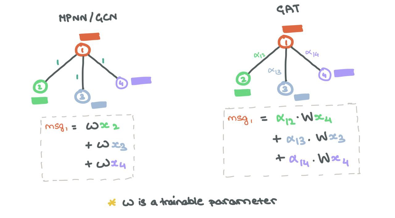
Edge Importance Weighting helps understand how much neighbours affects a source node.
As with the GCN, self-loops are added so source nodes can factor in their own representations for future representations.
GraphSAGE
Inductive Representation Learning on Large Graphs
GraphSAGE stands for Graph SAmple and AggreGatE. It’s a model to generate node embeddings for large, very dense graphs (to be used at companies like Pinterest).
The work introduces learned aggregators on a node’s neighbourhoods. Unlike traditional GATs or GCNs that consider all nodes in the neighbourhood, GraphSAGE uniformly samples the neighbours and uses the learned aggregators on them.
Suppose we have \(L\) layers in the network (depth), each layer \(l \in \{1,\dots,L\}\) looks at a larger \(l\)-hop neighbourhood w.r.t. the source node (as one would expect). Each source node is then updated by concatenating the node embedding with the sampled messages before being passed through a MLP \(F\) and non-linearity \(\sigma\).
For a certain layer \(l\),
\[h^l_{\mathcal{N}(i)} = \text{AGGREGATE}_{l}(\{h^{l-1}_j : j \in \mathcal{N}(i)\}) \\ h^l_i = \sigma(F(h^{l-1}_i ~\oplus~ h^l_{\mathcal{N}(i)}))\]where \(\oplus\) is the vector concatenation operation, and \(\mathcal{N}(i)\) is the uniform sampling function that returns a subset of all neighbours. So, if a node has 5 neighbours \(\{1,2,3,4,5\}\), possible outputs from \(\mathcal{N}(i)\) would be \(\{1,4,5\}\) or \(\{2,5\}\).
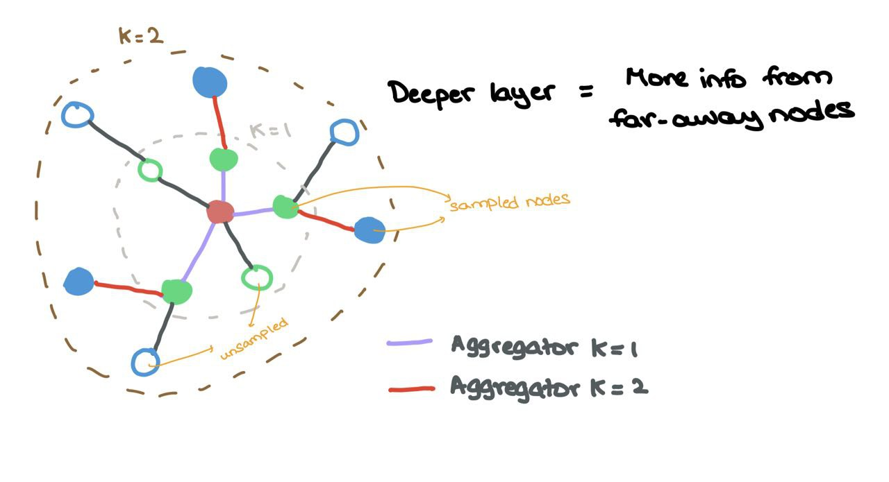
Aggregator \(k = 1\) aggregates sampled nodes (coloured) from the \(1\)-hop neighbourhood while Aggregator \(k = 2\) aggregates sampled nodes (coloured) from the \(2\)-hop neighbourhood
Possible future work could be experimenting with non-uniform sampling functions to choose neighbours.
Note: In the paper, the authors use \(K\) and \(k\) to denote the layer index. In this article, I use \(L\) and \(l\) respectively to stay consistent. Furthermore, the paper uses \(v\) to denomte source node \(i\) and \(u\) to denote neighbour \(j\).
Bonus: Prior work to GraphSAGE includes DeepWalk. Check it out!
Temporal Graph Network
Temporal Graph Networks for Deep Learning on Dynamic Graphs
The networks described so far work on static graphs. Most real-life situations work on dynamic graphs where nodes and edges are added, deleted, or updated over a duration of time. The Temporal Graph Network (TGN) has works on continuous time dynamic graphs (CTDG) that can be represented as a chronologically sorted list of events.
The paper breaks down events into two types: node-level events and interaction events. Node-level events involve a node in isolation (eg: a user updates their profile’s bio) while interaction events involve two nodes that may or may not be connected (eg: user A retweets/follows user B).
TGN offers a modular approach to CTDG processing with the following components:
Message Passing Function → message passing between isolated nodes or interacting nodes (for either type of event).
Message Aggregation Function → **uses the GAT’s aggregation by looking at a temporal neighbourhood through many timesteps instead of a local neighbourhood at a given timestep.
Memory Updater → memory allows the nodes to have long-term dependencies and represents the history of the node in latent (“compressed”) space. This module updates the node’s memory based on the interactions taking place through time.
Temporal Embedding → a way to represent the nodes that capture the essence of time as well.
Link prediction → the temporal embeddings of the nodes involves in an event are fed through some neural network to calculate edge probabilities (i.e., will the edge occur in the future?). Of course, during training, we know the edge exists so the edge label is \(1\). We need to train the Sigmoid-based network to predict this as usual.
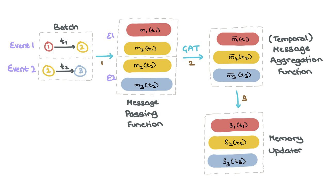
Every time a node is involved in an activity (node update or inter-node interaction), the memory is updated.
(1) For each event \(1\) and \(2\) in the batch, TGN generates messages for all nodes involved that event.
(2) Next, for TGN aggregates the messages of each node \(m_i\) for all timesteps \(t\); this is called the temporal neighbourhood of the node \(i\).
(3) Next, TGN uses the aggregated messages \(\bar{m}_i(t)\) to update the memory of each node \(s_i(t)\).
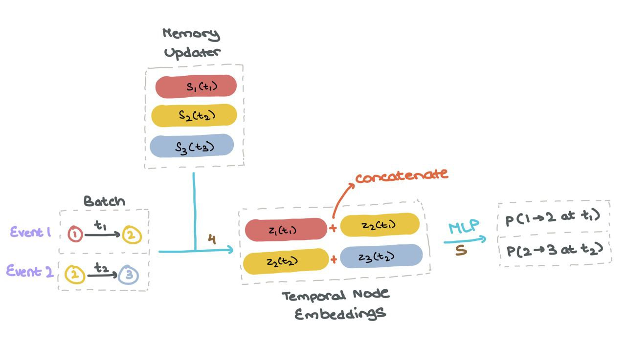
(4) Once the memory \(s_i(t)\) is up to date for all nodes, it’s used to compute “temporal node embeddings” \(z_i(t)\) for all nodes used in the specific interactions in the batch.
(5) These node embeddings are then fed into a MLP or neural network to get the probabilities of each the events taking place (using Sigmoid activation).
(6) We can then compute the loss using Binary Cross Entropy (BCE) as usual (not shown).
For more on the TGN, check out my short paper review here: Temporal Graph Networks for Deep Learning on Dynamic Graphs
The authors have also written a blogpost on the TGN that can be found here:
Conclusion
Graph Deep Learning is a great toolset when working with problems that have a network-like structure. They are simple to understand and implement using libraries like PyTorch Geometric, Spektral, Deep Graph Library, Jraph (if you use jax), and now, the recently-released TensorFlow-gnn. GDL has shown promise and will continue to grow as a field. In fact, most popular GDL papers come with a codebase written in either PyTorch or TensorFlow, so it helps a lot with experimentation.
Fun fact: GDL now falls under the umbrella of Geometric Deep Learning (“the new GDL”) that learns structural and spatial inductive biases on geometric surfaces like manifolds, graphs, and miscellaneous topologies. There are many academics who now specialise in Geometric DL with lots of exciting works coming out every month. In fact, I’d recommend taking a look at the dedicated Geometric Deep Learning course that features material by authors, Michael M. Bronstein, Joan Bruna, Taco Cohen, and Petar Veličković.
Till then, I’ll see you in the next post! Happy reading 😊
🙏🏻 If you want me to cover any of these papers or methods in more detail, email me at mail.rishabh.anand@gmail.com or DM me on Twitter at @rishabha16_.
Call To Action
If you like what you just read, there’s plenty more where that came from! Subscribe to my email newsletter / tech blog on Machine Learning and Technology:
Acknowledgements
I’d like to express my gratitude to Alex Foo and Chaitanya Joshi for the useful feedback and comments on this article. Our fruitful conversations and discussions shaped much of the work surrounding the GNN equations and their ease of readability. Thank you to Petar Veličković for his comments post-publication!